MATLABDiffEq.jl is a common interface binding for the MATLAB ordinary differential equation solvers. It uses the MATLAB.jl interop in order to
send the differential equation over to MATLAB and solve it. Note that this
package requires the differential equation function to be defined using
ParameterizedFunctions.jl.
Note that this package isn't for production use and is mostly just for benchmarking
and helping new users migrate models over to Julia.
For more efficient solvers, see the
DifferentialEquations.jl documentation.
Installation
To install MATLABDiffEq.jl, use the following:
using Pkg
Pkg.add("MATLABDiffEq")
Using MATLABDiffEq.jl
MATLABDiffEq.jl is simply a solver on the DiffEq common interface, so for details see the DifferentialEquations.jl documentation.
However, the only options implemented are those for error calculations
(timeseries_error), saveat and tolerances.
Note that the algorithms are defined to have the same name as the MATLAB algorithms,
but are not exported. Thus to use ode45, you would specify the algorithm as
MATLABDiffEq.ode45().
Example
using MATLABDiffEq, ParameterizedFunctions
f =@ode_def LotkaVolterra begin
dx =1.5x - x*y
dy =-3y + x*y
end
tspan = (0.0,10.0)
u0 = [1.0,1.0]
prob =ODEProblem(f,u0,tspan)
sol =solve(prob,MATLABDiffEq.ode45())
functionlorenz(du,u,p,t)
du[1] =10.0(u[2]-u[1])
du[2] = u[1]*(28.0-u[3]) - u[2]
du[3] = u[1]*u[2] - (8/3)*u[3]
end
u0 = [1.0;0.0;0.0]
tspan = (0.0,100.0)
prob =ODEProblem(lorenz,u0,tspan)
sol =solve(prob,MATLABDiffEq.ode45())
Measuring Overhead
To measure the overhead of over the wrapper, note that the variables
from the session will be still stored in MATLAB after the computation
is done. Thus you can simply call the same ODE function and time it
directly. This is done by:
To be even more pedantic, you can play around in the actual MATLAB
session by using
MATLABDiffEq.show_msession()
Overhead Amount
Generally, for long enough problems the overhead is minimal. Example:
using DiffEqBase, ParameterizedFunctions, MATLABDiffEq
f =@ode_def_bare RigidBodyBench begin
dy1 =-2*y2*y3
dy2 =1.25*y1*y3
dy3 =-0.5*y1*y2 +0.25*sin(t)^2end
prob =ODEProblem(f,[1.0;0.0;0.9],(0.0,100.0))
alg = MATLABDiffEq.ode45()
algstr =string(typeof(alg).name.name)
For this, we get the following:
julia>@time sol =solve(prob,alg);
0.063918 seconds (38.84 k allocations:1.556 MB)
julia>@time sol =solve(prob,alg);
0.062600 seconds (38.84 k allocations:1.556 MB)
julia>@time sol =solve(prob,alg);
0.061438 seconds (38.84 k allocations:1.556 MB)
julia>@time sol =solve(prob,alg);
0.065460 seconds (38.84 k allocations:1.556 MB)
julia>@time MATLABDiffEq.eval_string("[t,u] = $(algstr)(diffeqf,tspan,u0,options);")
0.058249 seconds (11 allocations:528 bytes)
julia>@time MATLABDiffEq.eval_string("[t,u] = $(algstr)(diffeqf,tspan,u0,options);")
0.060367 seconds (11 allocations:528 bytes)
julia>@time MATLABDiffEq.eval_string("[t,u] = $(algstr)(diffeqf,tspan,u0,options);")
0.060171 seconds (11 allocations:528 bytes)
julia>@time MATLABDiffEq.eval_string("[t,u] = $(algstr)(diffeqf,tspan,u0,options);")
0.058928 seconds (11 allocations:528 bytes)
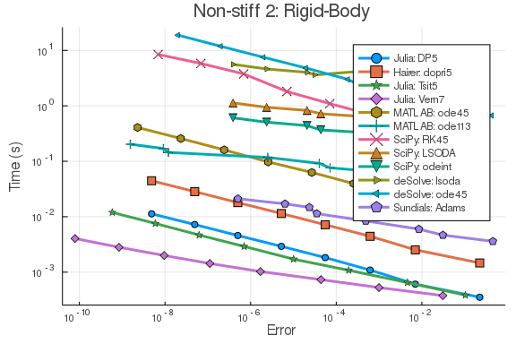
Benchmark
The following benchmarks demonstrate a 100x performance advantage for the
pure-Julia methods over the MATLAB ODE solvers across a range of stiff and
non-stiff ODEs. These were ran with Julia 1.2, MATLAB 2019B, deSolve 1.2.5,
and SciPy 1.3.1 after verifying negligible overhead on interop. Note that the
MATLAB solvers do outperform that of Python and R.
Non-Stiff Problem 1: Lotka-Volterra
f =@ode_def_bare LotkaVolterra begin
dx = a*x - b*x*y
dy =-c*y + d*x*y
end a b c d
p = [1.5,1,3,1]
tspan = (0.0,10.0)
u0 = [1.0,1.0]
prob =ODEProblem(f,u0,tspan,p)
sol =solve(prob,Vern7(),abstol=1/10^14,reltol=1/10^14)
test_sol =TestSolution(sol)
setups = [Dict(:alg=>DP5())
Dict(:alg=>dopri5())
Dict(:alg=>Tsit5())
Dict(:alg=>Vern7())
Dict(:alg=>MATLABDiffEq.ode45())
Dict(:alg=>MATLABDiffEq.ode113())
Dict(:alg=>SciPyDiffEq.RK45())
Dict(:alg=>SciPyDiffEq.LSODA())
Dict(:alg=>SciPyDiffEq.odeint())
Dict(:alg=>deSolveDiffEq.lsoda())
Dict(:alg=>deSolveDiffEq.ode45())
Dict(:alg=>CVODE_Adams())
]
names = [
"Julia: DP5""Hairer: dopri5""Julia: Tsit5""Julia: Vern7""MATLAB: ode45""MATLAB: ode113""SciPy: RK45""SciPy: LSODA""SciPy: odeint""deSolve: lsoda""deSolve: ode45""Sundials: Adams"
]
abstols =1.0./10.0.^ (6:13)
reltols =1.0./10.0.^ (3:10)
wp =WorkPrecisionSet(prob,abstols,reltols,setups;
names = names,
appxsol=test_sol,dense=false,
save_everystep=false,numruns=100,maxiters=10000000,
timeseries_errors=false,verbose=false)
plot(wp,title="Non-stiff 1: Lotka-Volterra")

 客服电话
客服电话
 APP下载
APP下载

 官方微信
官方微信


请发表评论