This repository covers how to prepare for machine learning interviews, mainly
in the format of questions & answers. Asides from machine learning knowledge,
other crucial aspects include:
Your resume should specify interesting ML projects you got involved in the past,
and quantitatively show your contribution. Consider the following comparison:
Trained a machine learning system
vs.
Trained a deep vision system (SqueezeNet) that has 1/30 model size, 1/3 training
time, 1/5 inference time, and 2x faster convergence compared with traditional
ConvNet (e.g., ResNet)
We all can tell which one is gonna catch interviewer's eyeballs and better show
case your ability.
In the interview, be sure to explain what you've done well. Spend some time going
over your resume before the interview.
SQL
Although you don't have to be a SQL expert for most machine learning positions,
the interviews might ask you some SQL related questions so it helps to refresh
your memory beforehand. Some good SQL resources are:
Given a data point, we compute the K nearest data points (neighbors) using certain
distance metric (e.g., Euclidean metric). For classification, we take the majority label
of neighbors; for regression, we take the mean of the label values.
Note for KNN technically we don't need to train a model, we simply compute during
inference time. This can be computationally expensive since each of the test example
need to be compared with every training example to see how close they are.
There are approximation methods can have faster inference time by
partitioning the training data into regions.
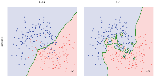
Note when K equals 1 or other small number the model is prone to overfitting (high variance), while
when K equals number of data points or other large number the model is prone to underfitting (high bias)
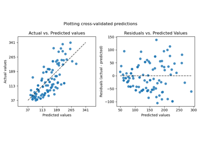
Given the training data, a decision tree algorithm divides the feature space into
regions. For inference, we first see which
region does the test data point fall in, and take the mean label values (regression)
or the majority label value (classification).
Construction: top-down, chooses a variable to split the data such that the
target variables within each region are as homogeneous as possible. Two common
metrics: gini impurity or information gain, won't matter much in practice.
Advantage: simply to understand & interpret, mirrors human decision making
Disadvantage:
can overfit easily (and generalize poorly)if we don't limit the depth of the tree
can be non-robust: A small change in the training data can lead to a totally different tree
instability: sensitive to training set rotation due to its orthogonal decision boundaries
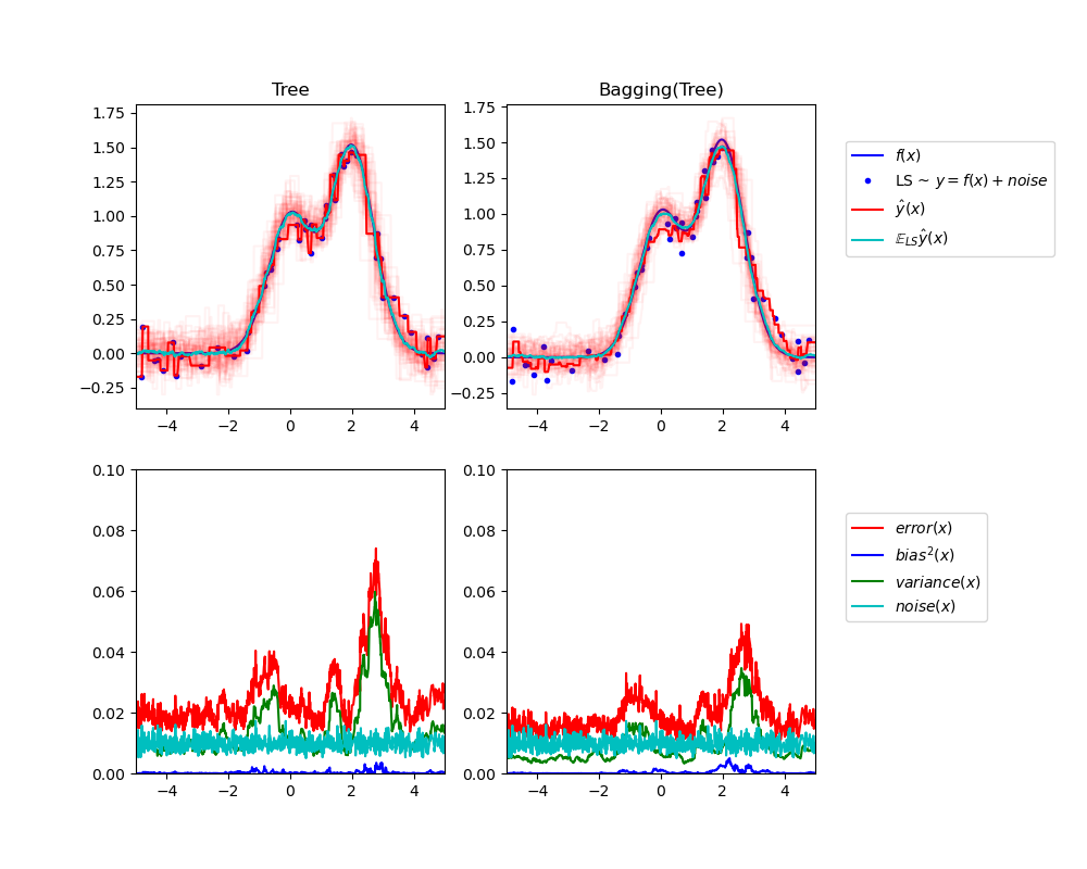
To address overfitting, we can use an ensemble method called bagging (bootstrap aggregating),
which reduces the variance of the meta learning algorithm. Bagging can be applied
to decision tree or other algorithms.
Random forest improves bagging further by adding some randomness. In random forest,
only a subset of features are selected at random to construct a tree (while often not subsample instances).
The benefit is that random forest decorrelates the trees.
For example, suppose we have a dataset. There is one very predicative feature, and a couple
of moderately predicative features. In bagging trees, most of the trees
will use this very predicative feature in the top split, and therefore making most of the trees
look similar, and highly correlated. Averaging many highly correlated results won't lead
to a large reduction in variance compared with uncorrelated results.
In random forest for each split we only consider a subset of the features and therefore
reduce the variance even further by introducing more uncorrelated trees.
In practice, tuning random forest entails having a large number of trees (the more the better, but
always consider computation constraint). Also, min_samples_leaf (The minimum number of
samples at the leaf node)to control the tree size and overfitting. Always CV the parameters.
Feature importance
In a decision tree, important features are likely to appear closer to the root of the tree. We can get
a feature's importance for random forest by computing the averaging depth at which it appears across all
trees in the forest.
Boosting builds on weak learners, and in an iterative fashion. In each iteration,
a new learner is added, while all existing learners are kept unchanged. All learners
are weighted based on their performance (e.g., accuracy), and after a weak learner
is added, the data are re-weighted: examples that are misclassified gain more weights,
while examples that are correctly classified lose weights. Thus, future weak learners
focus more on examples that previous weak learners misclassified.
Difference from random forest (RF)
RF grows trees in parallel, while Boosting is sequential
RF reduces variance, while Boosting reduces errors by reducing bias
XGBoost (Extreme Gradient Boosting)
XGBoost uses a more regularized model formalization to control overfitting, which gives it better performance
Instead of using trivial functions (such as hard voting) to aggregate the predictions from individual learners, train a model to perform this aggregation
First split the training set into two subsets: the first subset is used to train the learners in the first layer
Next the first layer learners are used to make predictions (meta features) on the second subset, and those predictions are used to train another models (to obtain the weigts of different learners) in the second layer
We can train multiple models in the second layer, but this entails subsetting the original dataset into 3 parts
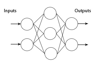
A feedforward neural network where we have multiple layers. In each layer we
can have multiple neurons, and each of the neuron in the next layer is a linear/nonlinear
combination of the all the neurons in the previous layer. In order to train the network
we back propagate the errors layer by layer. In theory MLP can approximate any functions.
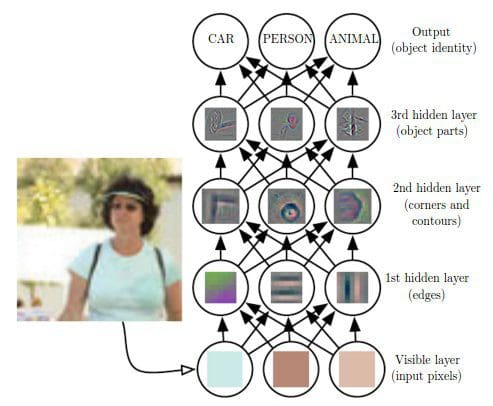
The Conv layer is the building block of a Convolutional Network. The Conv layer consists
of a set of learnable filters (such as 5 * 5 * 3, width * height * depth). During the forward
pass, we slide (or more precisely, convolve) the filter across the input and compute the dot
product. Learning again happens when the network back propagate the error layer by layer.
Initial layers capture low-level features such as angle and edges, while later
layers learn a combination of the low-level features and in the previous layers
and can therefore represent higher level feature, such as shape and object parts.
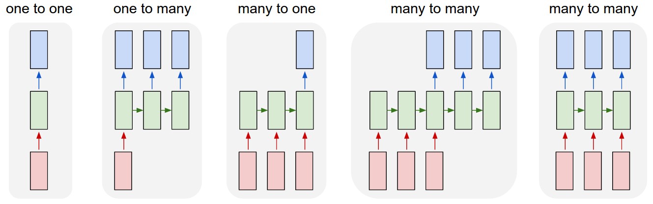
RNN is another paradigm of neural network where we have difference layers of cells,
and each cell only take as input the cell from the previous layer, but also the previous
cell within the same layer. This gives RNN the power to model sequence.
This seems great, but in practice RNN barely works due to exploding/vanishing gradient, which
is cause by a series of multiplication of the same matrix. To solve this, we can use
a variation of RNN, called long short-term memory (LSTM), which is capable of learning
long-term dependencies.
The math behind LSTM can be pretty complicated, but intuitively LSTM introduce
- input gate
- output gate
- forget gate
- memory cell (internal state)
LSTM resembles human memory: it forgets old stuff (old internal state * forget gate)
and learns from new input (input node * input gate)
Shallow, two-layer neural networks that are trained to construct linguistic context of words
Takes as input a large corpus, and produce a vector space, typically of several hundred
dimension, and each word in the corpus is assigned a vector in the space
The key idea is context: words that occur often in the same context should have same/opposite
meanings.
Two flavors
continuous bag of words (CBOW): the model predicts the current word given a window of surrounding context words
skip gram: predicts the surrounding context words using the current word
Discriminative algorithms model p(y|x; w), that is, given the dataset and learned
parameter, what is the probability of y belonging to a specific class. A discriminative algorithm
doesn't care about how the data was generated, it simply categorizes a given example
Generative algorithms try to model p(x|y), that is, the distribution of features given
that it belongs to a certain class. A generative algorithm models how the data was
generated.
Given a training set, an algorithm like logistic regression or
the perceptron algorithm (basically) tries to find a straight line—that is, a
decision boundary—that separates the elephants and dogs. Then, to classify
a new animal as either an elephant or a dog, it checks on which side of the
decision boundary it falls, and makes its prediction accordingly.
Here’s a different approach. First, looking at elephants, we can build a
model of what elephants look like. Then, looking at dogs, we can build a
separate model of what dogs look like. Finally, to classify a new animal, we
can match the new animal against the elephant model, and match it against
the dog model, to see whether the new animal looks more like the elephants
or more like the dogs we had seen in the training set.
A learning model that summarizes data with a set of parameters of fixed size (independent of the number of training examples) is called a parametric model.
A model where the number of parameters is not determined prior to training. Nonparametric does not mean that they have NO parameters! On the contrary, nonparametric models (can) become more and more complex with an increasing amount of data.

 客服电话
客服电话
 APP下载
APP下载

 官方微信
官方微信


请发表评论